Dating with FBD model tutorialAlexandra Gavryushkina |
1 Introduction
The tutorial illustrates how to use the BEAST software to co-estimate gene phylogenies and associated divergence times using fossil evidence and the fossilised birth-death (FBD) model [1]. The data required for such an analysis:
- Molecular data of extant species.
- Occurrence dates (or ranges) of fossil samples.
- Prior knowledge about the parameters of the FBD model. It could be a known proportion of sampled extant species, for example.
- Optionally, you can introduce monophyletic constraints on the phylogeny.
You will need the following software at your disposal:
- BEAST - this package contains the BEAST program, BEAUti, TreeAnnotator and other utility programs. This tutorial is written for BEAST v2.2.x. It is available for download from http://www.beast2.org/. A sampled ancestor (SA) package version 1.1.1 available for this version of BEAST supports sampled ancestor trees [1] and FBD model. The package can be installed through the package manager in BEAUti.
- Tracer - this program is used to explore the output of BEAST (and other Bayesian MCMC programs). It graphically and
quantitively summarizes the distributions of continuous parameters and provides diagnostic information. At the time of
writing, the current version is v1.6. It is available for download from
http://tree.bio.ed.ac.uk/software/. - FigTree - this is an application for displaying and printing molecular phylogenies, in particular those obtained using BEAST. At the time of writing, the current version is v1.4.2. It is available for download from http://tree.bio.ed.ac.uk/software/.
We assume that users are already familiar with basics of using BEAUti and BEAST.
2 Preparing the XML file
Having BEAST and SA package installed and sequence data of extant species together with empty sequences of fossil samples in a NEXUS file we can start preparing an XML file - the file which contains the specification of the analysis. First of all we need to upload the NEXUS file to BEAUti. In this tutorial, we use an example NEXUS file, bears.nex, which is available from the examples/nexus/ directory for Mac and Linux and examples\nexus\ for Windows inside the directory where SA package was installed. The package manager installs packages to
/Users/<YourName>/Library/Application Support/BEAST/2.2/ on Mac,
/home/<YourName>/.beast/2.2/ on Linux, and
Users\<YourName>\BEAST\2.2\ on Windows.
The example file contains an alignment of a single gene of ten extant species and 24 fossil samples (each site in the fossil sequences is a gap). After loading the alignment you may need to link trees and clock models if this is an alignment of multiple genes.
The next step is to specify the ages in the Tip Dates panel. Tick the ‘Use tip dates’ box. Then choose the right options in ‘Dates specified as’ section. We choose ‘years’ (the ages are given in My but a year is an appropriate unit since My is a decimal multiple of a year) and ‘Before the present’ options. Click on the ‘Guess’ button to load the dates from a separate file or extract the dates from taxon names or type in the dates directly to the cells of the table. In the example NEXUS file, the ages are included in the names of the taxa. So we choose ‘use everything after last _’ option to extract the dates (see Figure 1).

It is also possible to specify the age ranges however BEAUti does not support this option. If you want to do this then finish the XML specification in BEAUti and add the ranges manually. See bears_ranges.xml file in examples/ folder in the SA package directory as an example. Note that you still need to specify the ages in BEAUti. These ages should be within the ranges and will be used as initial values.
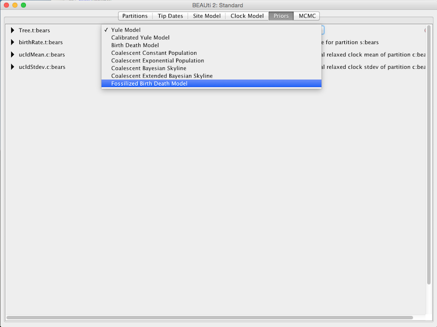
Further we need to specify site and clock models. We leave the default site model and choose the ‘Relaxed Clock Log Normal’ model with all default settings. Next we choose the ‘Fossilised Birth Death Model’ as the tree prior distribution (see Figure 2).
In the default settings of the FBD model, the proportion of species sampled at present, ρ, is fixed to one. For the example data, we leave this setting. In other analyses, you might need to change this value depending on the sampling scheme. Also you might choose another parameter to be fixed or estimate all the parameters placing informative prior distributions on one or more parameters. Although all the parameters in this model are identifiable, i.e., can be inferred from the phylogeny, in absence of comparative data of fossil samples we need to fix or place an informative prior distribution on one of the parameters. You also may need to adjust the initial values of the parameters, e.g., time of origin, which has to be older than the oldest fossil sample. If you believe all the fossil samples are crown, that is the most recent common ancestor of all taxa included in the analysis is not a fossil or, in other words, the root of the phylogeny is a two-degree node and not a sampled node, then also tick ‘Condition on Root’ box (see Figure 3). ‘Condition on Rho Sampling’ is preferable for a dating analysis and we leave it selected.

Further, you may specify monophyletic constraints on the same panel. Click the plus button at the bottom of the Priors panel, name the monophyletic clade and move all the taxa included in the clade to the right window. Then tick the ‘monophyletic’ box next to the ‘<Clade_name>.prior’ (Canidae.prior in the example) and leave the prior distribution as ‘[none]’ (see Figures 4 and 5). We do not recommend to specify any distribution for internal nodes because the interaction between multiple distributions applied to the phylogeny is not well understood.


Specify all the remaining prior distributions and proceed to the MCMC panel. We only change the ‘Log Every’ option for the ‘screenlog’ to 10000 to make the output of BEAST analysis more compact. Then save the file. Now the input XML file for BEAST is ready and you can run BEAST. The resulting XML file, bears.xml, prepared following this tutorial can be found in examples/ (or examples\ for Windows) directory in the SA package directory.
3 Analysing the results.
The output .log and .trees files will be in the same directory where the XML file is after the analysis is finished. Useful information is reported to the screen output. See this for information about the data, citations, and suggestions for improvement of the operator performance.
Open the LOG file in Tracer to review estimated statistics. For this analysis, the important parameters are the tree model parameters: origin, diversification rate, turnover and sampling proportion. Another statistic of interest is the sampled ancestor count (‘SAcountFBD’) which is the number of fossils that are direct ancestors of other fossils or extant taxa. Figure 6 shows the estimates of the model parameters and the posterior distribution for the number of sampled ancestors.

Use TreeAnnotator to summarise the tree distribution and FigTree to view the summary tree. The summary tree of trees in bears.trees is shown in Figure 7. It is obtained using TreeAnnotator with 10% burnin, zero ‘Posterior probability limit’, ‘Maximum Clade Credibility Tree’ as the ‘Target tree type’ and ‘Mean heights’ as ‘Node heights’. To find the maximum clade credibility tree the TreeAnnotator takes into account sampled ancestor clades, that is, any two clades with the same taxa are considered as distinct clades if the most recent common ancestor in one clade is a sampled node and in another clade is a bifurcation node. TreeAnnotator gives sensible results for sampled ancestor trees only in case when fossil ages are fixed.

References
- [1]
- A. Gavryushkina, D. Welch, T. Stadler, and A. J. Drummond. Bayesian inference of sampled ancestor trees for epidemiology and fossil calibration. PLoS Computational Biology, 10(12):e1003919, 2014.
This document was translated from LATEX by HEVEA.